Gradient Descent#
This is a supplement material for the Machine Learning Simplified book. It sheds light on Python implementations of the topics discussed while all detailed explanations can be found in the book.
I also assume you know Python syntax and how it works. If you don’t, I highly recommend you to take a break and get introduced to the language before going forward with my code.
This material can be downloaded as a Jupyter notebook (Download button in the upper-right corner ->
.ipynb) to reproduce the code and play around with it.
In the previous section we explored how to build a cost function in python. In this section, we will go further and explore each step of the gradient descent algorithm.
As a reminer, I’m leaving here our hypothetical dataset (Table 3.1) of six apartments located in the center of Amsterdam along with their prices (in 10,000 EUR) and floor areas (in square meters).
area (\(m^2\)) |
price (in €10,000) |
|---|---|
30 |
31 |
46 |
30 |
60 |
80 |
65 |
49 |
77 |
70 |
95 |
118 |
1. Required Libraries & Data#
Before we start, we need to import few libraries that we will use in this jupyterbook.
import sympy as sym #to take derivatives of functions
import matplotlib.pyplot as plt #to build graphs
import numpy as np #to work with numbers
%config InlineBackend.figure_format = 'retina' #to make sharper and prettier plots
Next step is to re-create our hypothetical dataset that we’ve been working with.
x = np.array([[30], [46], [60], [65], [77], [95]])
y = np.array([31, 30, 80, 49, 70, 118])
2. Gradient Descent in Action#
Let’s now see the gradient descent is action. But before we go into that, I’d like to recall how the fitted regression looks like - in other words, what regression the gradient needs to obtain in the end of its procedures.
In previous sections we understood that the function of the fitted regression is \(f(x) = -18 + 1.3*x\), let’s go ahead and plot this function using matplotlib library.
fig, ax = plt.subplots()

#plotting training dataset
ax.plot(x,y, 'o', color='g', label='training data')

#plotting the fitted regression
ax.plot(x, -18 + 1.3*x, label='y = {} + {} x'.format(-18, 1.3))

#showing legend and setting the size of the graph
plt.legend();
plt.ylim(0, 140)
plt.xlim(0, 110)
(0.0, 110.0)
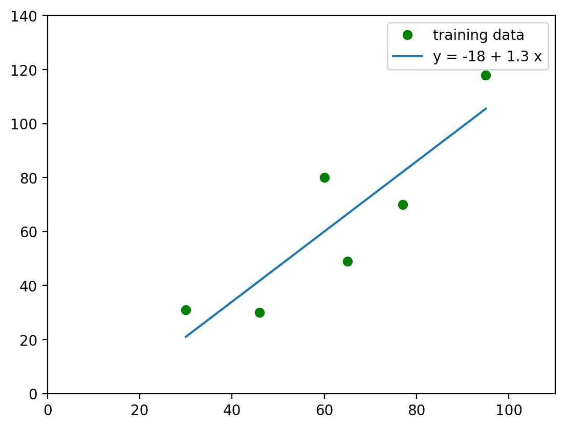
Ok, so the gradient descent needs to obtain identical regression as the one shown above. Visual representation is a nice thing, but we can also quantify the goodness of fit of this regression. Let’s calculate its Sum of Squared Residuals, or SSR, once again.
If you need a more detailed overview of how SSR is calculated, go to a previous section.
#preparing empty list for predicted values
y_pred = []

#simple loop to calculate each value predicted by the function, y_pred
for i in x:
    y_pred.append(-18 + 1.3*i)

print(y_pred)
[array([21.]), array([41.8]), array([60.]), array([66.5]), array([82.1]), array([105.5])]
#preparing empty list for residuals
r = []

#simple loop to calculate each redisual, r
for i in range(0, len(x)):
    r.append((y[i]-y_pred[i])**2)
print(r)
[array([100.]), array([139.24]), array([400.]), array([306.25]), array([146.41]), array([156.25])]
#sum all the residuals
ssr = np.sum(r)
print(ssr)
1248.1500000000003
2.1. Deriving Cost Function#
From previous sections we already know our cost function \(J(a)\):
\( \begin{equation} \begin{split} J(a) &= \sum\Big(y_i - (ax_i-18)\Big)^2 \\ &= \Big(31-(a*30-18)\Big)^2+\Big(30-(a*46-18)\Big)^2+\Big(80-(a*60-18)\Big)^2+\\ &+\Big(49-(a*65-18)\Big)^2+\Big(70-(a*77-18)\Big)^2+\Big(118-(a*95-18)\Big)^2 \end{split} \end{equation} \)
Let’s now take the derivative of this function with the respect to parameter \(a\). In python, you can simply derive any function using a special library sympy that we’ve already installed in the begining of this notebook.
# Calculating a derivative
a = sym.Symbol('a')
f = (31-(a*30-18))**2+(30-(a*46-18))**2+(80-(a*60-18))**2+(49-(a*65-18))**2+(70-(a*77-18))**2+(118-(a*95-18))**2
sym.diff(f)
Now that we have the derivative, gradient descent will use it to find where the Sum of Squared Residuals is the lowest.
2.2. Gradient Descent Steps#
Because the gradient descent does not know the true value of \(a\) that would minimize \(J(a)\) (which is \(a=1.3\)), it will start by setting \(a=0\).
2.2.1. Step 1#
First step is to plug \(a=0\) into the derivative:
a = 0
d = 51590*a-67218

print('Derivative = ', d)
Derivative = -67218
Thus, when \(a=0\), the slope of the curve = -67218 (which is identical to what we’ve received in the Machine Learning Simplified book).
Gradient descent use step size to get to the minimum point. Gradient descent determines the Step Size by multiplying the slope \(a\) by a small number called the learning rate \(l\).
Just like in the Machine Learning Simplified book, let’s take \(l=0.00001\) and calculate the Step Size:
\( \begin{equation} \begin{split} Step \ Size &= J(a) * l \\ &=(-67218)*0.00001 \end{split} \end{equation} \)
#setting the learning rate
l = 0.00001

#calculating step size
step_size = d*l

print('Step Size = ', step_size)
Step Size = -0.67218
And then we update \(a\): \( \begin{equation} \begin{split} a_{new} &= a - Step \ Size \\ &=0-(-0.67218)=0.67218 \end{split} \end{equation} \)
a1 = a-step_size
print('At Step 1, a = ', a)
At Step 1, a = 0
The first iteration is done. Let’s move forward.
2.2.2. Step 2#
Following the same logic, we now use the new coefficient \(a\) to calculate new derivative:
d = 51590*a1-67218
print('Derivative = ', round(d, 4))
Derivative = -32540.2338
step_size = d*l
print('Step Size = ', round(step_size, 5))
Step Size = -0.3254
a2 = a1-step_size
print('At Step 2, a = ', round(a2, 5))
At Step 2, a = 0.99758
2.2.3. Step 3#
d = 51590*a2-67218
print('Derivative = ', round(d, 4))
Derivative = -15752.7272
step_size = d*l
print('Step Size = ', round(step_size, 5))
Step Size = -0.15753
a3 = a2-step_size
print('At Step 3, a = ', round(a3, 5))
At Step 3, a = 1.15511
2.2.4. Step 4#
d = 51590*a3-67218
print('Derivative = ', round(d, 4))
Derivative = -7625.8952
step_size = d*l
print('Step Size = ', round(step_size, 5))
Step Size = -0.07626
a4 = a3-step_size
print('At Step 4, a = ', round(a4, 5))
At Step 4, a = 1.23137
2.2.5. Step 5#
d = 51590*a4-67218
print('Derivative = ', round(d, 4))
Derivative = -3691.6959
step_size = d*l
print('Step Size = ', round(step_size, 5))
Step Size = -0.03692
a5 = a4-step_size
print('At Step 5, a = ', round(a5, 5))
At Step 5, a = 1.26829
2.2.6. Step 6#
d = 51590*a5-67218
print('Derivative = ', round(d, 4))
Derivative = -1787.15
step_size = d*l
print('Step Size = ', round(step_size, 5))
Step Size = -0.01787
a6 = a5-step_size
print('At Step 6, a = ', round(a6, 5))
At Step 6, a = 1.28616
2.2.7. Step 7#
d = 51590*a6-67218
print('Derivative = ', round(d, 4))
Derivative = -865.1593
step_size = d*l
print('Step Size = ', round(step_size, 5))
Step Size = -0.00865
a7 = a6-step_size
print('At Step 7, a = ', round(a7, 5))
At Step 7, a = 1.29481
2.2.8. Step 8#
d = 51590*a7-67218
print('Derivative = ', round(d, 4))
Derivative = -418.8236
step_size = d*l
print('Step Size = ', round(step_size, 5))
Step Size = -0.00419
a8 = a7-step_size
print('At Step 8, a = ', round(a8, 5))
At Step 8, a = 1.299
2.2.9. Step 9#
d = 51590*a8-67218
print('Derivative = ', round(d, 4))
Derivative = -202.7525
step_size = d*l
print('Step Size = ', round(step_size, 5))
Step Size = -0.00203
a9 = a8-step_size
print('At Step 9, a = ', round(a9, 5))
At Step 9, a = 1.30102
2.2.10. Step 10#
d = 51590*a9-67218
print('Derivative = ', round(d, 4))
Derivative = -98.1525
step_size = d*l
print('Step Size = ', round(step_size, 5))
Step Size = -0.00098
a10 = a9-step_size
print('At Step 10, a = ', round(a10, 5))
At Step 10, a = 1.30201
2.2.11. Step 11#
d = 51590*a10-67218
print('Derivative = ', round(d, 4))
Derivative = -47.5156
step_size = d*l
print('Step Size = ', round(step_size, 5))
Step Size = -0.00048
a11 = a10-step_size
print('At Step 11, a = ', round(a11, 5))
At Step 11, a = 1.30248
2.2.12. Step 12#
d = 51590*a11-67218
print('Derivative = ', round(d, 4))
Derivative = -23.0023
step_size = d*l
print('Step Size = ', round(step_size, 5))
Step Size = -0.00023
a12 = a11-step_size
print('At Step 12, a = ', round(a12, 5))
At Step 12, a = 1.30271
2.2.13. Step 13#
d = 51590*a12-67218
print('Derivative = ', round(d, 4))
Derivative = -11.1354
step_size = d*l
print('Step Size = ', round(step_size, 5))
Step Size = -0.00011
a13 = a12-step_size
print('At Step 13, a = ', round(a13, 5))
At Step 13, a = 1.30282
2.2.14. Step 14#
d = 51590*a13-67218
print('Derivative = ', round(d, 4))
Derivative = -5.3907
step_size = d*l
print('Step Size = ', round(step_size, 5))
Step Size = -5e-05
a14 = a13-step_size
print('At Step 14, a = ', round(a14, 5))
At Step 14, a = 1.30288
2.2.15. Step 15#
d = 51590*a14-67218
print('Derivative = ', round(d, 4))
Derivative = -2.6096
step_size = d*l
print('Step Size = ', round(step_size, 5))
Step Size = -3e-05
a15 = a14-step_size
print('At Step 15, a = ', round(a15, 5))
At Step 15, a = 1.3029
Eventually, the gradient descent obtained the proper value for the parameter \(a = 1.3029\).
2.3. Different Initialization#
The gradient succeeded at finding the proper value for \(a\). Let’s now see what will happen if the gradient starts at a different value for \(a\), not \(a=0\). For instance, let’s take a random value of \(a=2.23\).
l = 0.00001 #same learning rate
a = 2.23 #different value for a
2.3.1. Step 1#
d = 51590*a-67218
print('Derivative = ', d)
Derivative = 47827.7
step_size = d*l
print('Step Size = ', step_size)
Step Size = 0.478277
a1 = a-step_size
print('At Step 1, a = ', round(a1, 5))
At Step 1, a = 1.75172
2.3.2. Step 2#
#step 2

d = 51590*a1-67218
print('Derivative = ', round(d, 4))

step_size = d*l
print('Step Size = ', round(step_size, 5))

a2 = a1-step_size
print('At Step 2, a = ', round(a2, 5))
Derivative =  23153.3896
Step Size =  0.23153
At Step 2, a =  1.52019
2.3.3. Step 3#
#step 3

d = 51590*a2-67218
print('Derivative = ', round(d, 4))

step_size = d*l
print('Step Size = ', round(step_size, 5))

a3 = a2-step_size
print('At Step 3, a = ', round(a3, 5))
Derivative =  11208.5559
Step Size =  0.11209
At Step 3, a =  1.4081
2.3.4. Step 4#
#step 4

d = 51590*a3-67218
print('Derivative = ', round(d, 4))

step_size = d*l
print('Step Size = ', round(step_size, 5))

a4 = a3-step_size
print('At Step 4, a = ', round(a4, 5))
Derivative =  5426.0619
Step Size =  0.05426
At Step 4, a =  1.35384
2.3.5. Step 5#
#step 5

d = 51590*a4-67218
print('Derivative = ', round(d, 4))

step_size = d*l
print('Step Size = ', round(step_size, 5))

a5 = a4-step_size
print('At Step 5, a = ', round(a5, 5))
Derivative =  2626.7566
Step Size =  0.02627
At Step 5, a =  1.32758
2.3.6. Step 6#
#step 6

d = 51590*a5-67218
print('Derivative = ', round(d, 4))

step_size = d*l
print('Step Size = ', round(step_size, 5))

a6 = a5-step_size
print('At Step 6, a = ', round(a6, 5))
Derivative =  1271.6129
Step Size =  0.01272
At Step 6, a =  1.31486
2.3.7. Step 7#
#step 7

d = 51590*a6-67218
print('Derivative = ', round(d, 4))

step_size = d*l
print('Step Size = ', round(step_size, 5))

a7 = a6-step_size
print('At Step 7, a = ', round(a7, 5))
Derivative =  615.5878
Step Size =  0.00616
At Step 7, a =  1.3087
2.3.8. Step 8#
#step 8

d = 51590*a7-67218
print('Derivative = ', round(d, 4))

step_size = d*l
print('Step Size = ', round(step_size, 5))

a8 = a7-step_size
print('At Step 8, a = ', round(a8, 5))
Derivative =  298.006
Step Size =  0.00298
At Step 8, a =  1.30572
2.3.9. Step 9#
#step 9

d = 51590*a8-67218
print('Derivative = ', round(d, 4))

step_size = d*l
print('Step Size = ', round(step_size, 5))

a9 = a8-step_size
print('At Step 9, a = ', round(a9, 5))
Derivative =  144.2647
Step Size =  0.00144
At Step 9, a =  1.30428
2.3.10. Step 10 - Step 15#
#step 10

d = 51590*a9-67218
print('Derivative = ', round(d, 4))

step_size = d*l
print('Step Size = ', round(step_size, 5))

a10 = a9-step_size
print('At Step 10, a = ', round(a10, 5))
Derivative =  69.8386
Step Size =  0.0007
At Step 10, a =  1.30358
#step 11

d = 51590*a10-67218
print('Derivative = ', round(d, 4))

step_size = d*l
print('Step Size = ', round(step_size, 5))

a11 = a10-step_size
print('At Step 10, a = ', round(a11, 5))
Derivative =  33.8088
Step Size =  0.00034
At Step 10, a =  1.30324
#step 12

d = 51590*a11-67218
print('Derivative = ', round(d, 4))

step_size = d*l
print('Step Size = ', round(step_size, 5))

a12 = a11-step_size
print('At Step 10, a = ', round(a12, 5))
Derivative =  16.3669
Step Size =  0.00016
At Step 10, a =  1.30308
#step 13

d = 51590*a12-67218
print('Derivative = ', round(d, 4))

step_size = d*l
print('Step Size = ', round(step_size, 5))

a13 = a12-step_size
print('At Step 10, a = ', round(a13, 5))
Derivative =  7.9232
Step Size =  8e-05
At Step 10, a =  1.303
#step 14

d = 51590*a13-67218
print('Derivative = ', round(d, 4))

step_size = d*l
print('Step Size = ', round(step_size, 5))

a14 = a13-step_size
print('At Step 10, a = ', round(a14, 5))
Derivative =  3.8356
Step Size =  4e-05
At Step 10, a =  1.30296
#step 15

d = 51590*a14-67218
print('Derivative = ', round(d, 4))

step_size = d*l
print('Step Size = ', round(step_size, 5))

a15 = a14-step_size
print('At Step 10, a = ', round(a15, 5))
Derivative =  1.8568
Step Size =  2e-05
At Step 10, a =  1.30294
The gradient descent successfully obtained the same proper value for the parameter \(a\), even though it was initialized with the different value for \(a\) in the beginning.