Decision Trees in Classification

• This is a supplement material for the Machine Learning Simplified book. It sheds light on Python implementations of the topics discussed while all detailed explanations can be found in the book.

• I also assume you know Python syntax and how it works. If you don’t, I highly recommend you to take a break and get introduced to the language before going forward with my code.

• This material can be downloaded as a Jupyter notebook (Download button in the upper-right corner -> .ipynb) to reproduce the code and play around with it.

This notebook is a supplement for Chapter 8. Decision Trees of Machine Learning For Everyone book.

1. Required Libraries, Data & Variables

Let’s import the data and have a look at it:

import pandas as pd
import matplotlib.pyplot as plt
%config InlineBackend.figure_format = 'retina' #to make sharper and prettier plots

# Creating the DataFrame based on the provided data
data = {
    'x1': [0.25, 0.60, 0.71, 1.20, 1.75, 2.26, 2.50, 2.50, 2.88, 2.91],
    'x2': [1.41, 0.39, 1.29, 2.30, 0.59, 1.70, 1.35, 2.90, 0.61, 2.00],
    'Color': ['blue', 'blue', 'blue', 'blue', 'blue', 'green', 'green', 'green', 'green', 'green']
}

# Convert the dictionary to a pandas DataFrame
df = pd.DataFrame(data)

# Display the DataFrame
df

	x1	x2	Color
0	0.25	1.41	blue
1	0.60	0.39	blue
2	0.71	1.29	blue
3	1.20	2.30	blue
4	1.75	0.59	blue
5	2.26	1.70	green
6	2.50	1.35	green
7	2.50	2.90	green
8	2.88	0.61	green
9	2.91	2.00	green

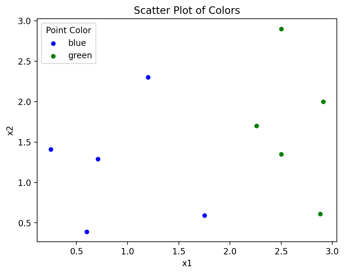
2. Visualizing Dataframe

# Plotting
fig, ax = plt.subplots()
colors = {'blue': 'blue', 'green': 'green'}

# Group by color and then plot each group
for key, group in df.groupby('Color'):
    group.plot(ax=ax, kind='scatter', x='x1', y='x2', label=key, color=colors[key])

# Setting plot labels and title
ax.set_xlabel('x1')
ax.set_ylabel('x2')
ax.set_title('Scatter Plot of Colors')

# Display the legend
ax.legend(title='Point Color')

# Show the plot
plt.show()

3. Preprocessing Dataframe

df['Color'] = df['Color'].map({'blue': 0, 'green': 1})

df

	x1	x2	Color
0	0.25	1.41	0
1	0.60	0.39	0
2	0.71	1.29	0
3	1.20	2.30	0
4	1.75	0.59	0
5	2.26	1.70	1
6	2.50	1.35	1
7	2.50	2.90	1
8	2.88	0.61	1
9	2.91	2.00	1

4. Training a Decision Tree with Gini

from sklearn.tree import DecisionTreeClassifier
from sklearn.model_selection import train_test_split
from sklearn.metrics import accuracy_score

4.1. Splitting into X and y

X = df[['x1', 'x2']]
y = df['Color']
X_train, X_test, y_train, y_test = train_test_split(X, y, test_size=0.2, random_state=42)

4.2. Building the Decision Tree Classifier

tree_classifier = DecisionTreeClassifier(criterion='gini', random_state=42)
tree_classifier.fit(X_train, y_train)

DecisionTreeClassifier(random_state=42)

In a Jupyter environment, please rerun this cell to show the HTML representation or trust the notebook.
On GitHub, the HTML representation is unable to render, please try loading this page with nbviewer.org.

4.3. Predict and Evaluate the Model

y_pred = tree_classifier.predict(X_test)
accuracy = accuracy_score(y_test, y_pred)
print("Accuracy of the decision tree model:", accuracy)

Accuracy of the decision tree model: 1.0

4.4. Visualize the Tree (optional)

from sklearn import tree
import graphviz

dot_data = tree.export_graphviz(tree_classifier, out_file=None, 
                                feature_names=['x1', 'x2'],  
                                class_names=['blue', 'green'],
                                filled=True, rounded=True,  
                                special_characters=True)  
graph = graphviz.Source(dot_data)  

# Visualize the decision tree
graph

5. Training a Decision Tree with Entropy

4.1. Splitting into X and y

X = df[['x1', 'x2']]
y = df['Color']
X_train, X_test, y_train, y_test = train_test_split(X, y, test_size=0.2, random_state=42)

4.2. Building the Decision Tree Classifier

tree_classifier = DecisionTreeClassifier(criterion='entropy', random_state=42)
tree_classifier.fit(X_train, y_train)

DecisionTreeClassifier(criterion='entropy', random_state=42)

In a Jupyter environment, please rerun this cell to show the HTML representation or trust the notebook.
On GitHub, the HTML representation is unable to render, please try loading this page with nbviewer.org.

4.3. Predict and Evaluate the Model

y_pred = tree_classifier.predict(X_test)
accuracy = accuracy_score(y_test, y_pred)
print("Accuracy of the decision tree model:", accuracy)

Accuracy of the decision tree model: 1.0

4.4. Visualize the Tree (optional)

from sklearn import tree
import graphviz

dot_data = tree.export_graphviz(tree_classifier, out_file=None, 
                                feature_names=['x1', 'x2'],  
                                class_names=['blue', 'green'],
                                filled=True, rounded=True,  
                                special_characters=True)  
graph = graphviz.Source(dot_data)  

# Visualize the decision tree
graph